PDF with Wigner and Q functions

Visualization of quantum states

from qutip import *
from qutip.distributions import *
import numpy as np
import matplotlib.pyplot as plt

Any photonic state or ensemble can be expressed in the fock basis. For example, a state $\psi\rangle$ is $$|\psi \rangle =\sum_{n}c_n |n\rangle $$ and an ensemble $\rho$ is $$ \rho =\sum_{m,n} \rho_{mn}|m\rangle\langle n| $$ where $|n\rangle$ is the number state with $n$ photons. The number $n$ ranges from $0$ to $\infty$. However, in computation, $n$ can not reach $\infty$. We set a maximum value $N_{\mathrm {max}}$.

Nmax = 25 # the maximum number of the fock state
rho_coherent = coherent_dm(Nmax, np.sqrt(4)) # create a coherent state with alpha = np.sqrrt(2)
rho_thermal = thermal_dm(Nmax, 3) # create a thermal state with <N> = 3
rho_fock = fock_dm(Nmax, 3) # create a fock state with n = 3
alpha = 3 
cat_state = coherent(Nmax,alpha) + coherent(Nmax,-alpha)
rho_cat = cat_state * cat_state.dag()

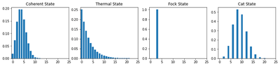
photon number counting

fig, axes = plt.subplots(1, 4, figsize=(15,3))
# plot the coherent state
bar0 = axes[0].bar(np.arange(0, Nmax), rho_coherent.diag())
lbl0 = axes[0].set_title("Coherent State")
lim0 = axes[0].set_xlim([-.5, Nmax])
# plot the thermal state
bar0 = axes[1].bar(np.arange(0, Nmax), rho_thermal.diag())
lbl0 = axes[1].set_title("Thermal State")
lim0 = axes[1].set_xlim([-.5, Nmax])
# plot the fock state
bar0 = axes[2].bar(np.arange(0, Nmax), rho_fock.diag())
lbl0 = axes[2].set_title("Fock State")
lim0 = axes[2].set_xlim([-.5, Nmax])
# plot the cat state
bar0 = axes[3].bar(np.arange(0, Nmax), rho_cat.diag())
lbl0 = axes[3].set_title("Cat State")
lim0 = axes[3].set_xlim([-.5, Nmax])
plt.show()

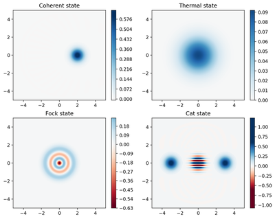
Wigner function

xvec = np.linspace(-5,5,200)
W_coherent = wigner(rho_coherent, xvec, xvec, g = 2) # g: scaling factor https://qutip.org/docs/latest/apidoc/functions.html#qutip.states.coherent
W_thermal = wigner(rho_thermal, xvec, xvec, g = 2)
W_fock = wigner(rho_fock, xvec, xvec, g = 2 )
W_cat = wigner(cat_state , xvec, xvec, g = 2)

# plot the results


fig, axes = plt.subplots(2, 2, figsize=(10,8), dpi=200)
cont0 = axes[0,0].contourf(xvec, xvec, W_coherent, 100,cmap='RdBu',vmin=-0.6, vmax=0.6)
lbl0 = axes[0,0].set_title("Coherent state")
plt.colorbar(cont0,ax=axes[0,0])
axes[0, 0].axis('equal')
#axes[0, 0].set(xlim=(-5, 5), ylim=(-5, 5))
cont1 = axes[0,1].contourf(xvec, xvec, W_thermal, 100,cmap='RdBu',vmin=-0.1, vmax=0.1)
lbl1 = axes[0,1].set_title("Thermal state")
plt.colorbar(cont1,ax=axes[0,1])
axes[0, 1].axis('equal')
cont2 = axes[1,0].contourf(xvec, xvec, W_fock, 100,cmap='RdBu',vmin=-0.6, vmax=0.6)
lbl2 = axes[1,0].set_title("Fock state")
plt.colorbar(cont2,ax=axes[1,0])
axes[1, 0].axis('equal')
cont3 = axes[1,1].contourf(xvec, xvec, W_cat, 100,cmap='RdBu',vmin=-0.6, vmax=0.6)
lbl3 = axes[1,1].set_title("Cat state")
plt.colorbar(cont3,ax=axes[1,1])
axes[1, 1].axis('equal')
plt.show()

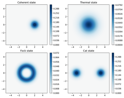
Husimi Q-function

xvec = np.linspace(-5,5,200)
Q_coherent = qfunc(rho_coherent, xvec, xvec, g = 2)
Q_thermal = qfunc(rho_thermal, xvec, xvec,g = 2)
Q_fock = qfunc(rho_fock, xvec, xvec, g = 2)
Q_cat = qfunc(cat_state , xvec, xvec, g = 2)

# plot the results

fig, axes = plt.subplots(2, 2, figsize=(10,8),dpi=200)
cont0 = axes[0,0].contourf(xvec, xvec, Q_coherent, 100,cmap='RdBu',vmin=-0.3, vmax=0.3)
lbl0 = axes[0,0].set_title("Coherent state")
plt.colorbar(cont0,ax=axes[0,0])
axes[0, 0].axis('equal')
axes[0, 0].set(xlim=(-5, 5), ylim=(-5, 5))
cont1 = axes[0,1].contourf(xvec, xvec, Q_thermal, 100,cmap='RdBu',vmin=-0.08, vmax=0.08)
lbl1 = axes[0,1].set_title("Thermal state")
plt.colorbar(cont1,ax=axes[0,1])
axes[0, 1].axis('equal')
cont2 = axes[1,0].contourf(xvec, xvec, Q_fock, 100,cmap='RdBu',vmin=-0.08, vmax=0.08)
lbl2 = axes[1,0].set_title("Fock state")
plt.colorbar(cont2,ax=axes[1,0])
axes[1, 0].axis('equal')
cont3 = axes[1,1].contourf(xvec, xvec, Q_cat, 100,cmap='RdBu',vmin=-0.3, vmax=0.3)
lbl3 = axes[1,1].set_title("Cat state")
plt.colorbar(cont3,ax=axes[1,1])
axes[1, 1].axis('equal')
plt.show()