Harmonic Ocsillator
We show how to compute the harmonic oscillator in the number basis. We use the quantum toolbox in Python, qutip.
from qutip import *
from qutip.distributions import *
import numpy as np
import matplotlib.pyplot as plt
We begin with the number basis. ‘a = destroy()’ genrerates the annillation operator in the numner basis.
$$ a = \begin{pmatrix} 0 & 0 & 0&\dots\\
1 & 0 & 0&\dots\\
0 &\sqrt{2}&0&\dots\\
0 & 0 &\sqrt{3} &\ddots
\end{pmatrix} $$
Then, we write $x$ and $p$ operators in the number basis,
$$ x = \frac{a+a^{\dagger}}{2}, \
p = \frac{a-a^{\dagger}}{2i},$$
and compute the eigenbasis of $x$ operator, that is, to express $|x_i\rangle$ in the number basis.
## create the operators in the number basis (Fock basis)
N = 501 # the maximum number of the photon number
a = destroy(N)
x = (a + a.dag())/2
p = (a - a.dag())/2j

# to find the basis vectors of x operator (but expressed in the number basis)
x_vals, x_states = x.eigenstates()
Discussion here is more advanced. You can skip this part.
The problem here is related to the gauge fixing of the phase. Since the phases of the eigenstates can be arbitrary, there exist the degree of freedom to add the phase $$ |x_\mathrm{new} \rangle = \exp{i\phi(x)}|x \rangle,$$ where $\phi(x)$ is an arbitrary funciton. When we obtain $|x\rangle $ numerically, it may occur that $\phi(x)$ is not a continuous funciton of $x$. The discontinuity will cause problems, says when computing the derivatives of wavefunctions with respect to $x$. Below, we remedy the issue.
The basis vectors $|x_i\rangle$ by ‘x_states’ are obtained by the exact diagonalization of the $x$ matrix. A typical problem of numerically obtained $|x_i\rangle$ is that the phase of different $|x_i\rangle$ is not continuous in $x$. This leads to the problem of discontinuities of $\psi(x)$. To fix this problem, we require the following condition $$\mathrm{Arg}[\langle x_{i+1}|p|x_i\rangle]= \frac{\pi}{2}. $$
#  The x_states contains the eigenvectors. However, the phase of each eigenvector is not continuous
#  as a function of xi.
#  This casuses a problem that the wavefunciton psi(x) is not continuous.
# # The way to remedy the issue is to make <xi+1|p|xi> have the same phase
x_states[0] = - x_states[0] # to fix the phase such that psi_0(x) >0
for i in range(N-1):
    tmp1 = x_states[i+1].dag()*p*x_states[i]
    ph = np.angle(tmp1)
    ph_c = np.pi/2 - ph[0,0]
    x_states[i+1] = np.exp(1j* ph_c)* x_states[i+1]
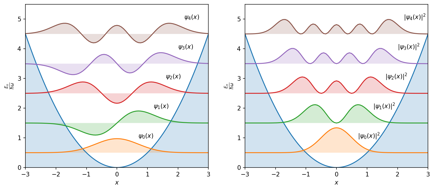
## plot the harmonic potential V = 1/2 x^2

plt.figure(dpi=150,figsize=(12,5))
# subplot 1
plt.subplot(1,2,1)
plt.plot(x_vals, x_vals**2/2)
plt.fill_between(x_vals, 0., x_vals**2/2, alpha=0.2)
## plot the probabilities of the eigenstates
for i in range(5):
    psi = fock(N,i) ## fock states are the eigenstates of a harmonic oscillator
    Ei = 1/2 + i
    psi_x = psi.transform(x_states)
    y1 = np.abs(psi_x.full())**2 * 15 + Ei
    y1 = np.real(psi_x.full()) * 2 + Ei
    y1 = np.reshape(y1,(N,))
    plt.plot(x_vals, y1)
    plt.fill_between(x_vals, Ei, y1 , alpha=0.2)
plt.ylabel(r"$\frac{E_n}{\hbar\omega}$")
plt.xlabel(r"$x$")
plt.xlim([-3,3])
plt.ylim([0,5.5])
plt.text(0.7,1, '$\psi_0(x)$')
plt.text(1.2,2, '$\psi_1(x)$')
plt.text(1.6,3, '$\psi_2(x)$')
plt.text(2,4, '$\psi_3(x)$')
plt.text(2.2,5, '$\psi_4(x)$');

# subplot 2
plt.subplot(1,2,2)
plt.plot(x_vals, x_vals**2/2)
plt.fill_between(x_vals, 0., x_vals**2/2, alpha=0.2)
## plot the probabilities of the eigenstates
for i in range(5):
    psi = fock(N,i) ## fock states are the eigenstates of a harmonic oscillator
    Ei = 1/2 + i
    psi_x = psi.transform(x_states)
    y1 = np.abs(psi_x.full())**2 * 15 + Ei
    y1 = np.reshape(y1,(N,))
    plt.plot(x_vals, y1)
    plt.fill_between(x_vals, Ei, y1 , alpha=0.2)
plt.ylabel(r"$\frac{E_n}{\hbar\omega}$")
plt.xlabel(r"$x$")
plt.xlim([-3,3])
plt.ylim([0,5.5])
plt.text(0.7,1, '$|\psi_0(x)|^2$')
plt.text(1.2,2, '$|\psi_1(x)|^2$')
plt.text(1.6,3, '$|\psi_2(x)|^2$')
plt.text(2,4, '$|\psi_3(x)|^2$')
plt.text(2.2,5, '$|\psi_4(x)|^2$');
from qutip.ipynbtools import version_table
version_table()
| Software | Version |
|---|---|
| QuTiP | 4.6.3 |
| Numpy | 1.22.2 |
| SciPy | 1.8.0 |
| matplotlib | 3.4.0 |
| Cython | 0.29.28 |
| Number of CPUs | 8 |
| BLAS Info | OPENBLAS |
| IPython | 8.1.1 |
| Python | 3.10.2 | packaged by conda-forge | (main, Feb 1 2022, 19:29:00) [GCC 9.4.0] |
| OS | posix [linux] |
| Sun Mar 06 16:06:18 2022 CST | |
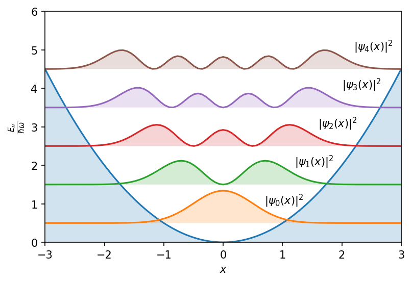
Instead of using the Fock states (number states), we compute the eigenstates dierectly from the hamiltonians. Of course, we will obtain the same results.
hamil =  x**2 + p**2
en_vals, h_states = hamil.eigenstates()
plt.figure(dpi=150)
plt.plot(x_vals, x_vals**2/2)
plt.fill_between(x_vals, 0., x_vals**2/2, alpha=0.2)

## plot the probabilities of the eigenstates

for i in range(5):
    Ei = 1/2 + i
    psi_x = h_states[i].transform(x_states)
    y1 = np.abs(psi_x.full())**2 * 15 + Ei
    y1 = np.reshape(y1,(N,))
    plt.plot(x_vals, y1)
    plt.fill_between(x_vals, Ei, y1 , alpha=0.2)

plt.ylabel(r"$\frac{E_n}{\hbar\omega}$")
plt.xlabel(r"$x$")
plt.xlim([-3,3])
plt.ylim([0,6])
plt.text(0.7,1, '$|\psi_0(x)|^2$')
plt.text(1.2,2, '$|\psi_1(x)|^2$')
plt.text(1.6,3, '$|\psi_2(x)|^2$')
plt.text(2,4, '$|\psi_3(x)|^2$')
plt.text(2.2,5, '$|\psi_4(x)|^2$');